14 Style Guide

Using a consistent style across your projects can increase the overhead as your data science team discusses options, decides on a good choice, and develops in compliant code. But like in most themes in this document, the cost is worth the effort. Unforced code errors are reduced when code is consistent, because mistake-prone styles are more apparent.

For the most part, our team follows the tidyverse style. Here are some additional conventions we attempt to follow. Many of these were inspired by (Francesco Balena 2005).

14.1 Readability

14.1.1 Number

The word “number” is ambiguous, especially in data science. Try for these more specific terms:

• count: the number of discrete objects or events, such as visit_count, pt_count, dx_count.
• id: a value that uniquely identifies an entity that doesn’t change over time, such as pt_id, clinic_id, client_id,
• index: a 1-based sequence that’s typically temporary, but unique within the dataset. For instance, pt_index 195 in Tuesday’s dataset is like;y a different person than pt_index 195 on Wednesday. On any given day, there is only one value of 195.
• tag: it is persistent across time like “id”, but typically created by the analysts and send to the research team. See the snippet in the appendix for an example.
• tally: a running count
• duration: a length of time. Specify the units if it not self-evident.
• physical and statistical quantities like “depth”, “length”, “mass”, “mean”, and “sum”.

14.1.2 Abbreviations

Try to avoid abbreviations. Different people tend to shorten words differently; this variability increases the chance that people reference the wrong variable. At very least, it wastes time trying to remember if subject_number, subject_num, or subject_no was used. The Consistency section describes how this can reduce errors and increase efficiency.

However, some terms are too long to reasonably use without shortening. We make some exceptions, such as the following scenarios:

1. humans commonly use the term orally. For instance, people tend to say “OR” instead of “operating room”.

2. your team has agreed on set list of abbreviations. The list for our CDW team includes: appt (not “apt”), cdw, cpt, drg (stands for diagnosis-related group), dx, hx, icd pt, and vr (vital records).

When your team choose terms (e.g., ‘apt’ vs ‘appt’), try to use a standard vocabulary, such as MedTerms Medical Dictionary.

14.2 Datasets

14.2.1 Filtering Rows

Removing datasets rows is an important operation that is a frequent source of sneaky errors. These practices reduce our mistakes and improve maintainability.

14.2.1.1 Mimic number line

When ordering quantities, go smallest-to-largest as you type left-to-right. At minimum be consistent with the direction. In other words, use operators like < and <= and avoid > and >=. This approach also makes it more consistent with the SQL and dplyr function, between().

# Good (b/c quantities increase as you read left-to-right)
ds_teenager |>
  dplyr::filter(13 <= age & age < 20)

# Not as good (b/c quantities increase as you read right-to-left)
ds_teenager |>
  dplyr::filter(20 > age & age <= 13)

# Bad (b/c the order is inconsistent)
ds_teenager |>
  dplyr::filter(age >= 13 & age < 20)
ds_teenager |>
  dplyr::filter(age < 20 & age >= 13)

14.2.1.2 Searchable verbs

You’ve occasionally asked in frustration, “Where did the dataset lose some rows? It had 900 rows in the middle of the script, but now has only 782.” You then scan through the script for any location that potentially removes rows. These locations are easier to identify when you’re scanning for only a small set of filtering functions such as tidyr::drop_na(), dplyr::filter(), and dplyr::summarize(). You can even highlight them with ‘ctrl+f’. In contrast, the base R’s filtering style is more difficult to identify.

# tidyverse's approach is easy to see in a long script
ds <-
  ds |>
  dplyr::filter(4 <= count)
  
# base R's approach is harder to see
ds <- ds[4 <= ds$count, ]

14.2.1.3 Remove rows with missing values

Even within tidyverse functions, there are preferences in certain scenarios. This entry covers the scenario of dropping an entire row if an important column is missing a value.

tidyr::drop_na() removes rows with a missing value in a specific column. It is cleaner to read and write dplyr’s filter() and base R’s subsetting bracket. In particular, it’s easy to forget/overlook a !.

# Cleanest
ds |>
  tidyr::drop_na(dob)

# Not as good
ds |>
  dplyr::filter(!is.na(dob))

# Ripest for mistakes or misinterpretation
ds[!is.na(ds$dob), ]

14.2.2 Don’t attach

As the Google Stylesheet says, “The possibilities for creating errors when using attach() are numerous.”

Hopefully you’ve learned R recently enough that you haven’t read examples from the 1990s that used attach(). It may have made sense in the early days of S-PLUS when the language was used primarily interactively by a single statistician. But the contemporary tradeoffs are unfavorable, now that R scripts are frequently run by multiple people and functions are run in multiple contexts.

14.3 Categorical Variables

There are lots of names for a categorical variable across the different disciplines (e.g., factor, categorical, …).

14.3.1 Explicit Missing Values

Define a level like "unknown" so the data manipulation doesn’t have to test for both is.na(x) and x == "unknown". The explicit label also helps when included in a statistical procedure and coefficient table.

14.3.2 Granularity

Sometimes it helps to represent the values differently, say with a granular variable and a coarse variable. If two related variables have 7 and 3 levels respectively, we say *_cut7 and *_cut3 to denote the resolution; this is related to base::cut(). Don’t forget to include “unknown” and “other” when necessary.

# Inside a dplyr::mutate() clause
education_cut7      = dplyr::recode(
  education_cut7,
  "No Highschool Degree / GED"  = "no diploma",
  "High School Degree / GED"    = "diploma",
  "Some College"                = "some college",
  "Associate's Degree"          = "associate",
  "Bachelor's Degree"           = "bachelor",
  "Post-graduate degree"        = "post-grad",
  "Unknown"                     = "unknown",
  .missing                      = "unknown",
),
education_cut3      = dplyr::recode(
  education_cut7,
  "no diploma"    = "no bachelor",
  "diploma"       = "no bachelor",
  "some college"  = "no bachelor",
  "associate"     = "no bachelor",
  "bachelor"      = "bachelor",
  "post-grad"     = "bachelor",
  "unknown"       = "unknown",
),
education_cut7 = factor(education_cut7, levels=c(
  "no diploma",
  "diploma",
  "some college",
  "associate",
  "bachelor",
  "post-grad",
  "unknown"
)),
education_cut3 = factor(education_cut3, levels=c(
  "no bachelor",
  "bachelor",
  "unknown"
)),

The dplyr::recode_factor() is an ideal replacement in the scenario above, because a single call combines the work of dplyr::recode() and base::factor(). Just make sure the recoding order represents the desired order of the factor levels.

# Inside a dplyr::mutate() clause
education_cut7      = dplyr::recode_factor(
  education_cut7,
  "No Highschool Degree / GED"  = "no diploma",
  "High School Degree / GED"    = "diploma",
  "Some College"                = "some college",
  "Associate's Degree"          = "associate",
  "Bachelor's Degree"           = "bachelor",
  "Post-graduate degree"        = "post-grad",
  "Unknown"                     = "unknown",
  .missing                      = "unknown",
),
education_cut3      = dplyr::recode_factor(
  education_cut7,
  "no diploma"    = "no bachelor",
  "diploma"       = "no bachelor",
  "some college"  = "no bachelor",
  "associate"     = "no bachelor",
  "bachelor"      = "bachelor",
  "post-grad"     = "bachelor",
  "unknown"       = "unknown",
),

14.4 Dates

Date arithmetic is hard. Naming dates well might be harder.

• birth_month_index can be values 1 through 12, while birth_month (or commonly mob) contains the year (e.g., 2014-07-15).

• birth_year is an integer, but birth_month and birth_week are dates. Typically months are collapsed to the 15th day and weeks are collapsed to Monday, which are the defaults of OuhscMunge::clump_month_date() and OuhscMunge::clump_week_date(). These obfuscate the real value when PHI is involved. Months are centered because the midpoint is usually a better representation of the month’s performance than the month’s initial day.

• Don’t use the minus operator (i.e., -). See Defensive Date Arithmetic.

14.5 Naming

14.5.1 Variables

This builds upon the tidyverse style guide for objects.

14.5.1.1 Characters

Use lowercase letters, using underscores to separate words. Avoid uppercase letters and periods.

14.5.2 Semantic Order

For variables including multiple nouns or adjectives, place the more global terms before the more microscopic terms. The “bigger” term goes first; the “smaller” terms are successively nested in the bigger terms.

# Good:
parent_name_last
parent_name_first
parent_dob
kid_name_last
kid_name_first
kid_dob

# Bad:
last_name_parent
first_name_parent
dob_parent
last_name_kid
first_name_kid
dob_kid

Large datasets with multiple questionnaires (each with multiple subsections) are much more manageable when the variables follow a semantic order.

SELECT
  asq3_medical_problems_01
  ,asq3_medical_problems_02
  ,asq3_medical_problems_03
  ,asq3_behavior_concerns_01
  ,asq3_behavior_concerns_02
  ,asq3_behavior_concerns_03
  ,asq3_worry_01
  ,asq3_worry_02
  ,asq3_worry_03
  ,wai_01_steps_beneficial
  ,wai_02_hv_useful
  ,wai_03_parent_likes_me
  ,wai_04_hv_doubts
  ,hri_01_client_input
  ,hri_02_problems_discussed
  ,hri_03_addressing_problems_clarity
  ,hri_04_goals_discussed
FROM miechv.gpav_3

I don’t know where we picked up the term “semantic order”. It may have come from Semantic Versioning of software releases.

14.5.3 Files and Folders

Naming files and their folders/directories follows the style of naming variables, with one small difference: separate words with dashes (i.e., -), not underscores (i.e., _). In other words, “kebab case” instead of “snake case.

Occasionally, we’ll use a dash if it helps identify a noun (that already contains an underscore). For instance, if there’s a table called patient_demographics, we might call the files patient_demographics-truncate.sql and patient_demographics-insert.sql.

Using lower case is important because some databases and operating systems are case-sensitive, and some are case-insensitive. To promote portability, keep everything lowercase.

Again, file and folder names should contain only (a) lowercase letters, (b) digits, (c) dashes, and (d) an occasional dash. Do not include spaces, uppercase letters, and especially punctuation, such as : or (.

14.5.4 Datasets

tibbles (which are fancy data.frames) are used in almost every analysis file, so we put extra effort formulating conventions that are informative and consistent. Naming datasets follows the style of naming variables, with a few additional features.

In the R world, “dataset” is typically a synonym of data.frame –a rectangular structure of rows and columns. The database equivalent is a conventional table. Note that “dataset” means a collections of tables in the the .NET world, and a collection of (not-necessarily-rectangular) files in Dataverse.⁹

14.5.4.1 Prefix with ds_ and d_

Datasets are handled so differently than other variables that we find it’s easier to identify its type and scope. The prefix ds_ indicates the dataset is available to the entire file, while d_ indicates the scope is localized to a function.

count_elements <- function (d) {
  nrow(d) * ncol(d)
}

ds <- mtcars
count_elements(d = ds)

14.5.4.2 Express the grain

The grain of a dataset describes what each row represents, which is a similar idea to the statistician’s concept of “unit of analysis”. Essentially it the the most granular entity described. Many miscommunications and silly mistakes are avoided when your team is disciplined enough to define a tidy dataset with a clear grain.

ds_student          # One row per student
ds_teacher          # One row per teacher
ds_course           # One row per course
ds_course_student   # One row per student-course combination

ds_pt         # One row per patient
ds_pt_visit   # One row per patient-visit combination
ds_visit      # Same as above, since it's clear a visit is connected w/ a pt

For more insight into grains, Ralph Kimball writes

In debugging literally thousands of dimensional designs from my students over the years, I have found that the most frequent design error by far is not declaring the grain of the fact table at the beginning of the design process. If the grain isn’t clearly defined, the whole design rests on quicksand. Discussions about candidate dimensions go around in circles, and rogue facts that introduce application errors sneak into the design. … I hope you’ve noticed some powerful effects from declaring the grain. First, you can visualize the dimensionality of the doctor bill line item very precisely, and you can therefore confidently examine your data sources, deciding whether or not a dimension can be attached to this data. For example, you probably would exclude “treatment outcome” from this example because most medical billing data doesn’t tie to any notion of outcome.

14.5.4.3 Singular table names

If you adopt the style that the table’s name reflects the grain, this is a corollary. If the grain is singular like “one row per client” or “one row per building”, the name should be ds_client and ds_building (not ds_clients and ds_buildings). If these datasets are saved to a database, the tables are called client and building.

Table names are plural when the grain is plural. If a record has field like client_id, date_birth, date_graduation and date_death, I suggest called the table client_milestones (because a single row contains three milestones).

This Stack Overflow post presents a variety of opinions and justifications when adopting a singular or plural naming scheme.

I think it’s acceptable if the R vectors follow a different style than R data.frames. For instance, a vector can have a plural name even though each element is singular (e.g., client_ids <- c(10, 24, 25)).

14.5.4.4 Use ds when definition is clear

Many times an ellis file handles with only one incoming csv and outgoing dataset, and the grain is obvious –typically because the ellis filename clearly states the grain.

In this case, the R script can use just ds instead of ds_county.

14.5.4.5 Use an adjective after the grain, if necessary

If the same R file is manipulating two datasets with the same grain, qualify their differences after the grain, such as ds_client_all and ds_client_michigan. Adjectives commonly indicate that one dataset is a subset of another.

An occasional limitation with our naming scheme is that the difficult to distinguish the grain from the adjective. For instance, is the grain of ds_student_enroll either (a) every instance of a student enrollment (i.e., student and enroll both describe the grain) or (b) the subset of students who enrolled (i.e., student is the grain and enroll is the adjective)? It’s not clear without examine the code, comments, or documentation.

If someone has a solution, we would love to hear it. So far, we’ve been reluctant to decorate the variable name more, such as ds_grain_client_adj_enroll.

14.5.4.6 Define the dataset when in doubt

If it’s potentially unclear to a new reader, use a comment immediately before the dataset’s initial use. The grain is frequently the most important characteristic to document.

# `ds_client_enroll`:
#    grain: one row per client
#    subset: only clients who have successfully enrolled are included
#    source: the `client` database table, where `enroll_count` is 1+.
ds_client_enroll <- ...

14.6 Whitespace

Although execution is rarely affected by whitespace in R and SQL files, be consistent and minimalistic. One benefit is that Git diffs won’t show unnecessary churn. When a line of code lights up in a diff, it’s nice when reflect a real change, and not something trivial like tabs were converted to spaces, or trailing spaces were added or deleted.

Some of these guidelines are handled automatically by modern IDEs, if you configure the correct settings.

1. Tabs should be replaced by spaces. Most modern IDEs have an option to do this for you automatically. (RStudio calls this “Insert spaces for tabs”.)
2. Indentions should be replaced by a consistent number of spaces, depending on the file type.
   1. R: 2 spaces
   2. SQL: 2 spaces
   3. Python: 4 spaces
3. Each file should end with a blank line. (The RStudio checkbox is “Ensure that source files end with newline.”)
4. Remove spaces and tabs at the end of lines.
   • VS Code: see the VS Code section of the Workstation chapter.
   • Azure Data Studio: See the ADS section of the Workstation chapter.
   • RStudio: Global Options | Code | Saving | Strip trailing horizontal whitespace when saving.
   • SSMS:

14.7 Database

GitLab’s data team has a good style guide for databases and sql that’s fairly consistent with our style. Some important additions and differences are

1. Favor CTEs over subqueries because they’re easier to follow and can be reused in the same file. If the performance is a problem, slightly rewrite the CTE as a temp table and see if it and the new indexes help.

   Resources:

   • Brent Ozar’s SQL Server Common Table Expressions defines the basics:

     A CTE effectively creates a temporary view that a developer can reference multiple times in the underlying query.

   • Brent Ozar’s What’s Better, CTEs or Temp Tables? The article’s bottom line is:

     I’d suggest starting with CTEs because they’re easy to write and to read. If you hit a performance wall, try ripping out a CTE and writing it to a temp table, then joining to the temp table.

2. The name of the primary key should typically contain the table. In the employee table, the key should be employee_id, not id.

14.8 Code Repositories

Our analytical team dedicates a private repo to each research project. It is a repository in GitHub accessible only to the team members granted explicit privileges. Repos are also discussed in the Git & GitHub appendix.

14.8.1 Repo Naming

As of 2022, our GitHub organization has 300 repos. Many of them are focused warehouse projects that are completed within a month. The easiest and most stable naming system we’ve found is built from three parts:

1. PI’s last name. Even if we are in contact with only the project manager, we prefer to use the primary investigator’s name (typically the name on the IRB application) because it rarely changes and it is easier to trace to the right team. Do not refer to a medical resident or fellow that will rotate out in a few months.
2. Two or three word term. Describe the global area in a few words.
3. Index. Be optimistic and prepare for follow up investigations. The initial repo is “…-1”, the subsequent repos are “…-2, …-3, …-4”.

# Good Examples
akande-asthma-hospitalization-1
akande-asthma-hospitalization-2
akande-covid-1
bard-covid-1
bard-covid-2
bard-eeg-education-1

# Bad Examples
akande-1
akande-2
covid-1
covid-2
covid-3
bard-research-1

We informally call this the “project tag” and try to use it consistently in different arenas, such as:

• The GitHub repo’s name.
• The parent directory for the project on the file server (e.g., M:/pediatrics/bbmc/akande-covid-1).
• The database schema containing the project’s tables (e.g., akande_covid_1.patient, akande_covid_1.visit, akande_covid_2.visit). Change from kebab case to snake case (e.g., akande-covid-1 to akande_covid_1) so the sql code doesn’t have to escape the schema name with brackets.
• In the body of emails to help retrospective searches.

14.8.2 Repo Granularity

The boundaries of a research project may be fuzzy, so you may not have a clear answer to the question, “should this be considered one large research project with one repo, or two smaller research projects with two total repos?”. The deciding factor for us is usually determined by the amount of living code that would need to exist in both repos. If the two projects are being developed in parallel and you would have to make similar changes in both repos, strongly consider using only one repo.

Other issues that suggest a unified repo:

• The two repos have almost identical users.
• The two repos are covered by the same IRB.

Issues that suggest separate repos:

• The development windows don’t overlap. If the initial project wrapped up last year and a follow-up study is starting, consider a separate repo that starts with a subset of the code. Start fresh and copy over only what’s necessary

14.8.3 Repo Pricing

We enrolled in some GitHub program in 2012 that allows academic research group to have unlimited private repos in the GitHub Organization. Otherwise, it would not be feasible to have 300+ tightly-focused repos.

GitHub seems to introduce new programs or modify existing branding every few years. The current best documentation is “Apply for an educator or researcher discount”. Notice this program is more more lightweight than a program like “GitHub Campus”, which involves your whole campus apparently.

14.9 ggplot2

The expressiveness of ggplot2 allows someone to quickly develop precise scientific graphics. One graph can be specified in many equivalent styles, which increases the opportunity for confusion. We formalized much of this style while writing a textbook for introductory statistics (Lise DeShea (2015)); the 200+ graphs and their code is publicly available.

There are a few additional ggplot2 tips in the tidyverse style guide.

14.9.1 Order of commands

ggplot2 is essentially a collection of functions combined with the + operator. Publication graphs common require at least 20 functions, which means the functions can sometimes be redundant or step on each other toes. The family of functions should follow a consistent order ideally starting with the more important structural functions and ending with the cosmetic functions. Our preference is:

1. ggplot() is the primary function to specify the default dataset and aesthetic mappings. Many arguments can be passed to aes(), and we prefer to follow an order consistent with the scale_*() order below.
2. geom_*() and annotate() creates the geometric elements that represent the data. Unlike most categories in this list, the order matters. Geoms specified first are drawn first, and therefore can be obscured by subsequent geoms.
3. scale_*() describes how a dimension of data (specified in aes()) is translated into a visual element. We specify the dimensions in descending order of (typical) importance: x, y, group, color, fill, size, radius, alpha, shape, linetype.
4. coord_*()
5. facet_*() and label_*()
6. guides()
7. theme() (call the ‘big’ themes like theme_minimal() before overriding the details like theme(panel.grid = element_line(color = "gray")))
8. labs()

This graph contains most typical ggplot2 elements.

ggplot(ds, aes(x = group, y = lift_count, fill = group, color = group)) +
  geom_bar(stat = "summary", fun.y = "mean", color = NA) +
  geom_point(position = position_jitter(w = 0.4, h = 0), shape = 21) +
  scale_color_manual(values = palette_pregnancy_dark) +
  scale_fill_manual( values = palette_pregnancy_light) +
  coord_flip() +
  facet_wrap("time") +
  theme_minimal() +
  theme(legend.position = "none") +
  theme(panel.grid.major.y = element_blank()) +
  labs(
    title = "Lifting by Group across Time"
    x     = NULL, 
    y     = "Number of Lifts"
  )

14.9.2 Gotchas

Here are some common mistakes we see not-so-infrequently (even sometimes in our own ggplot2 code).

14.9.2.1 Zooming

Call coord_*() to restrict the plotted x/y values, not scale_*() or lims()/xlim()/ylim(). coord_*() zooms in on the axes, so extreme values essentially fall off the page; in contrast, the latter three functions essentially remove the values from the dataset. The distinction does not matter for a simple bivariate scatterplot, but likely will mislead you and the viewer in two common scenarios. First, a call to geom_smooth() (e.g., that overlays a loess regression curve) ignore the extreme values entirely; consequently the summary location will be misplaced and its standard errors too tight. Second, when a line graph or spaghetti plots contains an extreme value, it is sometimes desirable to zoom in on the the primary area of activity; when calling coord_*(), the trend line will leave and return to the plotting panel (which implies points exist which do not fit the page), yet when calling the others, the trend line will appear interrupted, as if the extreme point is a missing value.

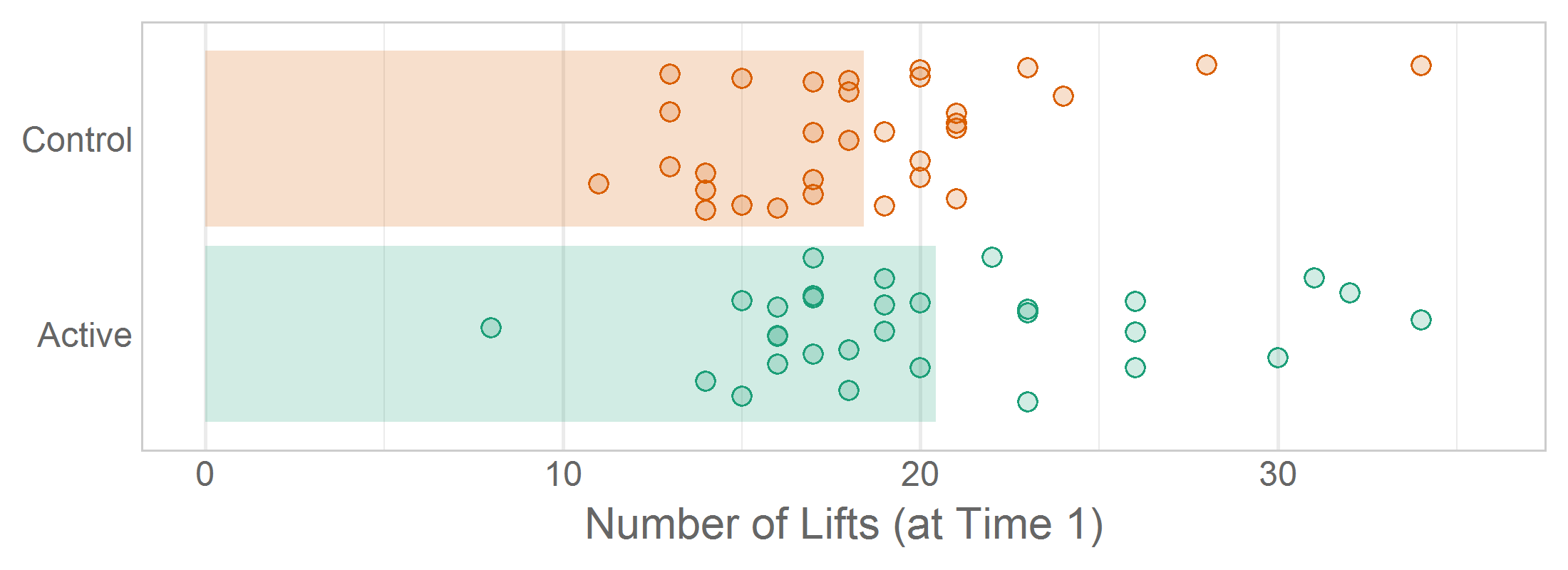
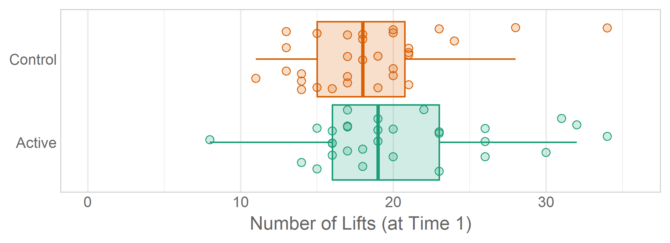
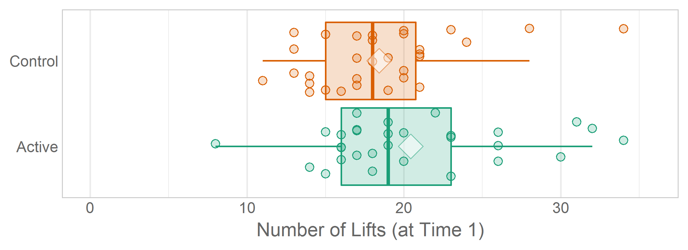
14.9.2.2 Seed

When jittering, set a seed in the ‘declare-globals’ chunk so that rerunning the report won’t create a (slightly) different png. The insignificantly different pngs will consume extra space in the Git repository. Also, the GitHub diff will show the difference between png versions, which requires extra subjectivity and cognitive load to determine if the difference is due solely to jittering, or if something really changed in the analysis.

# ---- declare-globals ---------------------------------------------------------
set.seed(seed = 789) # Set a seed so the jittered graphs are consistent across renders.

Occasionally you’ll want multiple graphs in the same report to have a consistent jitter, so set the same seed prior to each ggplot() call. In Lise DeShea’s 2015 book, Figures 3-21, 3-22, and 3-23 needed to be as similar as possible so the inter-graph differences were easier to distinguish.

# ---- figure-03-21 ------------------------------------------------------
set.seed(seed = 789)
ggplot(ds, aes(x = group, y = t1_lifts, fill = group)) +
...

# ---- figure-03-22 ------------------------------------------------------
set.seed(seed = 789)
ggplot(ds, aes(x = group, y = t1_lifts, fill = group)) +
...

# ---- figure-03-23 ------------------------------------------------------
set.seed(seed = 789)
ggplot(ds, aes(x = group, y = t1_lifts, fill = group)) +
...